How To Change What A Pivot Tables Colum Filter Is Called

Filters in Pin tables are not similar like filters in the tables or information nosotros use, in pivot table filters we have 2 methods to employ filters, one is past right click on the pin table and we will find the filter option for the pivot tabular array filter, another method is by using the filter options provided in the pivot tabular array fields.

How to Filter in a Pivot Tabular array?

The pin table is a user-friendly spreadsheet tool in excel which allows united states of america to summarize, grouping, perform mathematical operations similar SUM, AVERAGE, COUNT, etc. from the organized data that is stored in a database. Apart from the mathematical operations, the Pivot table got one of the best features, i.east., filtering, which allows usa to excerpt defined results from our data.

Let's look at multiple ways of using a filter in an Excel Pin table: –

#1 – Inbuilt filter in the Excel Pivot Table

Permit'due south have the data in one of the worksheets.

Pivot table Filter examplee 1.1

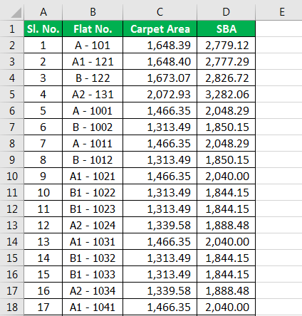
The above information consists of 4 different columns with S.No, Flat no's, Rug Expanse & SBA.

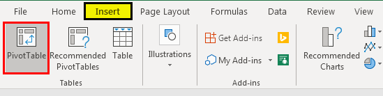
Get to the insert tab and select a Pivot table, equally shown below.

Pivot table Filter examplee 1.2

When you click on the pivot tabular array, the "Create a Pin Table" window pops out.

Pivot table Filter examplee 1.3

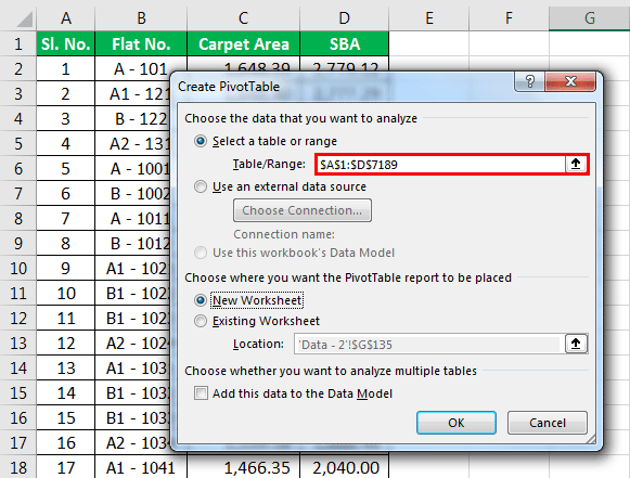
In this window, we have got an selection of selecting a tabular array or a range to create a pivot table, or nosotros likewise can apply an external data source too.

We as well have the option of placing the Pin table report, whether in the same worksheet or new worksheet, and we tin see this in the above picture.

Pin table Field will exist bachelor on the right end of the sheet as below.

Pivot table Filter examplee 1.4

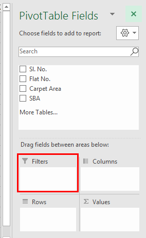
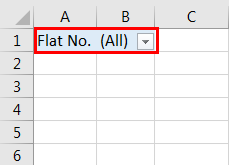
Nosotros can observe the filter field, where we can drag the fields into filters to create a Pivot table filter. Let'south drag the Flat no's field into Filters, and we tin can run across the filter for Flat no'southward would take been created.

Pivot table Filter examplee 1.5

From this, we can filter the Flat no'southward as per our requirement, and this is the normal style of creating the filter in the Pin table.

Pivot table Filter examplee 1.6

#ii – Create a filter to Values Area of an Excel Pivot table

Mostly, when we take data into value areas, there won't be any filter created to those Pin Table fields Pivot table calculated fields are formulas with reference to other fields, and calculated values refer to other values within a specific pivot field. read more . Nosotros tin can see it beneath.

Pivot table Filter examplee 2.1

Pivot table Filter examplee 2.2

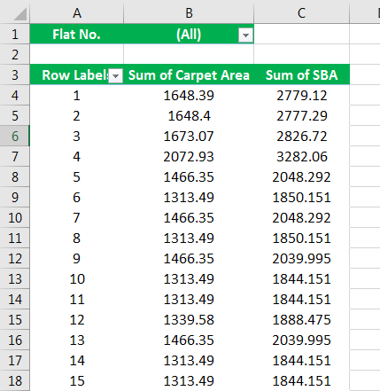
We can clearly find that there is no filter option for value areas, i.e., Sum of SBA & Sum of Carpet Area. Simply we can really create it and which helps us in various decision-making purposes.

Firstly, we have to select any cell next to the table and click on the filter in the data tab.

Pivot table Filter examplee 2.3

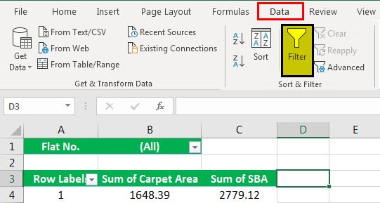
We tin see the filter gets in the value areas.

Pivot table Filter examplee 2.4

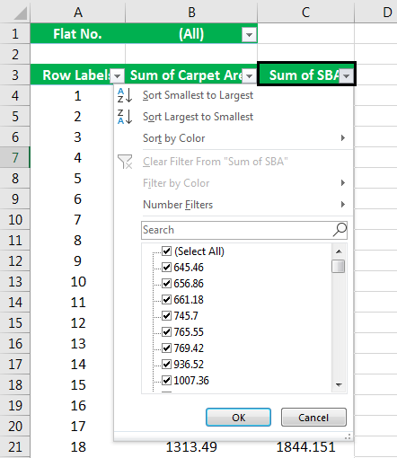
As we got the filters, we tin can now perform unlike types of operations from value areas as well, similar sorting them from largest to smallest in order to know top sales/surface area/anything. Similarly, nosotros can do sorting from smallest to largest, sorting by color, and even we tin perform number filters like <=,<,>=,>, and many more. This plays a major role in decision-making in any arrangement.

#3 – Display a list of multiple items in a Pivot Table Filter.

In the higher up example, we had learned of creating a filter in the Pivot Table. Now allow's look at the way we brandish the list in different ways.

3 most important ways of displaying a list of multiple items in a pivot table filter are: –

Using Slicers.
Creating a list of cells with filter criteria.
List of Comma Separated Values.

Using Slicers

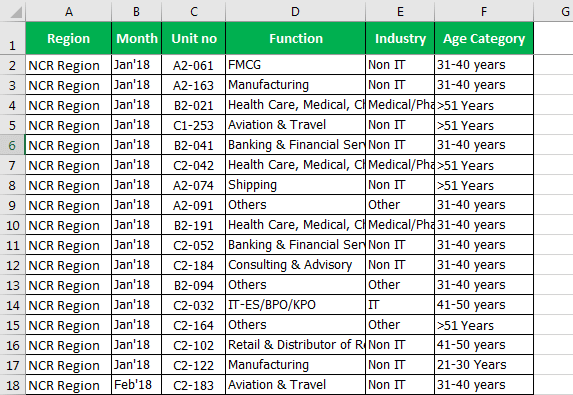
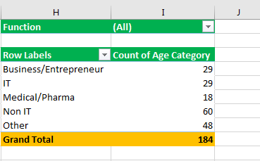
Let'due south have a simple pin table with different columns like Region, Month, Unit no, Function, Manufacture, Historic period Category.

example 3.1

Offset, create a pivot table using the above-given data. Select the data, then get to the insert tab and select a pivot table option and create a pivot tabular array.

example 3.2

example 3.4

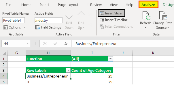
From this example, we are going to consider Function in our filter, and let'southward bank check how it tin can be listed using slicers and varies as per our pick. It is simple as we simply select any cell inside the pivot tabular array, and nosotros'll get to the analyze tab on the ribbon and choose the insert slicer.

example 3.3

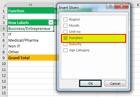
So we're going to insert the slide the slicer of the filed in our filter expanse, so in this case, the "Office" filed in our filter area and then striking Ok, and that's going to add together a slicer to the sheet.

example 3.5

Nosotros tin run across items that are highlighted in the slicer are those which are highlighted in our Pin Tabular array filter criteria in the filter drop-down menu.

example 3.6

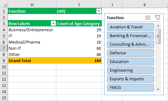
Now, this is a pretty elementary solution that does brandish the filter criteria. By this, we can easily filter out multiple items and can run into the result varying in value areas. From the beneath instance, it is clear that we had selected the functions that are visible in the slicer and can find out the count of age category for different Industries (which are row labels that we had dragged into the row label field) which are associated with those part that is in a slicer. We tin alter the function as per our requirement and tin observe the results vary as per the items selected.

Yet, if you lot have a lot of items in your list here and it'south really long, and so those items might not be displayed properly, and yous might accept to do a lot of scrolling to see which items are selected, so that leads us to the nest solution of listing out the filter criteria in cells.

Then, "Create List of cells with Pivot Table Filter Criteria" comes to our rescue.

Create Listing of cells with Pin Table Filter Criteria: –

Nosotros're going to use a continued pivot tabular array, and nosotros're basically going to use the higher up slicer here to connect two pivot tables together.

Now let us create a duplicate copy of the existing pivot table and paste it into a blank cell.

example 4.1

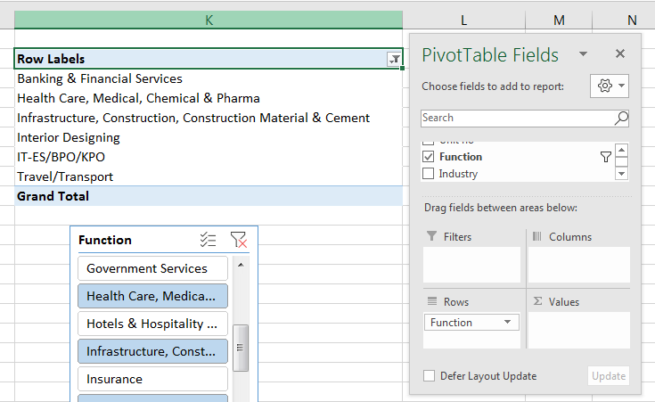
And then now nosotros have a indistinguishable copy of our pivot table, and nosotros are going to alter a little fleck to show that Functions field in the rows area.

To do this, we have to select whatever cell within of our pivot table here and go over to the pin table field list and going to remove Industry from the rows, removing Count of Age Category from the values area, and nosotros are going to take the Part that is in our filters area to rows area, and and then now we can see that nosotros have a listing of our filter criteria if we look over hither in our filter drib-downward card we have the list of particular that is there in slicers and function filter too.

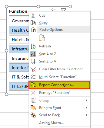
Now we have a list of our pivot table filter criteria, and this works because both of these pivot tables are continued past the slicer. If nosotros correct-click anywhere on the slicer & to study connections

example 4.2

Pivot table connections that will open upwards a menu that shows us that both of these pivot tables are connected every bit checkboxes are checked.

example 4.3

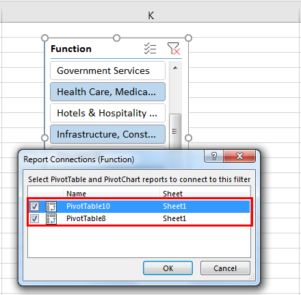
This means whenever 1 inverse is fabricated in 1st pivot, information technology would automatically go reflected in the other.

Tables tin be moved anywhere; information technology tin exist used in any financial models; row labels tin also be changed.

List of Comma Separated Values in Excel Pivot Table Filter: –

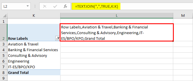
So the third way to display our pivot table filter criteria is in a single jail cell with a list of comma-separated values, and we tin can do that with the TEXTJOIN function. We still need the tables that we used earlier and simply used a formula to create this string of values and separate them with commas.

This is a new formula or new role that was introduced in Excel 2016 & it's chosen TEXTJOIN(If there is no 2016, you can use concatenate function also); text joining makes this procedure much easier.

TEXTJOIN basically gives the states three dissimilar arguments

Delimiter – which tin can be a comma or space
Ignore empty – true or false to ignore empty cells or non
Text – add together or specify a range of cells they contain the values we want to concatenate

Let's blazon TEXTJOIN – (delimiter- which would exist "," in this case, TRUE (as we should ignore empty cells), K: Chiliad(similar the listing of selected items from the filter will be available in this column)to join any value & likewise ignore whatever empty value)

Pivot table Filter example 5.1

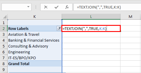
Now we see getting a list of all of our pivot table filter criteria joined by a string. And so it's basically a comma-separated listing of values.

Pivot table Filter example 5.2

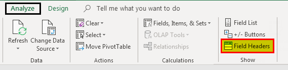
If nosotros didn't want to show these filter criteria in the formula, we could hide the jail cell. Just select the prison cell and become up to the analyze options tab; click on field headers & that will hide the cell.

Pivot table Filter example 5.3

Pivot table Filter example 5.4

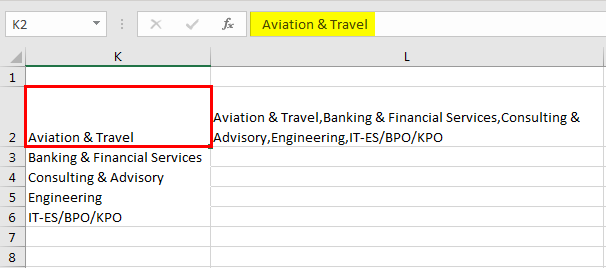
So now nosotros have the list of values in their Pivot Table filter criteria. Now, if we make changes in the pivot table filter, it reflects in all the methods. We can employ whatsoever one of there. Just somewhen, for comma-separated solution slicer & the list is required. If you don't want to display the tables, they can be subconscious.

Things to remember nearly Excel Pin Table Filter

Pivot Table Filtering is not an additive because when we select one criterion and if we want to filter again with other criteria, so the first 1 will get discarded.
We got a special characteristic in the Pivot Table filter, i.east., "Search Box," which allows us to deselect manually some of the results that we don't want. For Ex: If we take got a huge list and there are blanks too, then in order to select bare, we tin can easily get selected by searching for blank in the search box rather than scrolling down till the end.
Nosotros are not supposed to exclude certain results with a condition in the Pivot Table filter, only nosotros can practise it by using the "label filter." For Ex: If we want to select any product with a certain currency like rupee or dollar, etc., then we tin can use a label filter – 'does not contain' and should give the status.

You tin can download this Excel Pin table filter template from here – Pivot Table Filter Excel Template.

Recommended Manufactures

This has been a guide to the Pin table filter in Excel. Here we discuss how to Filter Data in a Pivot tabular array with the assist of examples and a downloadable excel template. You lot may larn more near excel from the following articles –